Inference for Means & Confidence Interval for µ

STAT 218 - Week 4, Lecture 3

Inference for Means

Important Symbols

To distinguish a quantitative variable from a categorical variable, we use different symbols to show population parameters and sample statistics.

Parameters

\(\mu\) = population mean

\(\sigma\) = population standard deviation

Statistics

\(\bar{x}\) = sample mean

\(s\) = sample standard deviation

College Midwest - Example

Let’s consider a situation (again) where we actually have access to the entire population.
We recently obtained data on the student body of a small college in the Midwest.
- There are 2,919 students in this population.
- We will take a random sample of 30 students.

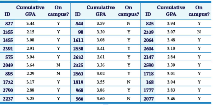
Observational Unit: A student in that college. Variable: Cumulative GPA Statistic: Sample Mean

College Midwest - Example

Each simple random sample gave us a different value for the sample mean. Taking 1,000 random samples helps us see the long-run pattern to these statistics.
- In other words, we are approximating the sampling distribution of the sample means.
Let’s see the applet to conduct a hypothesis testing

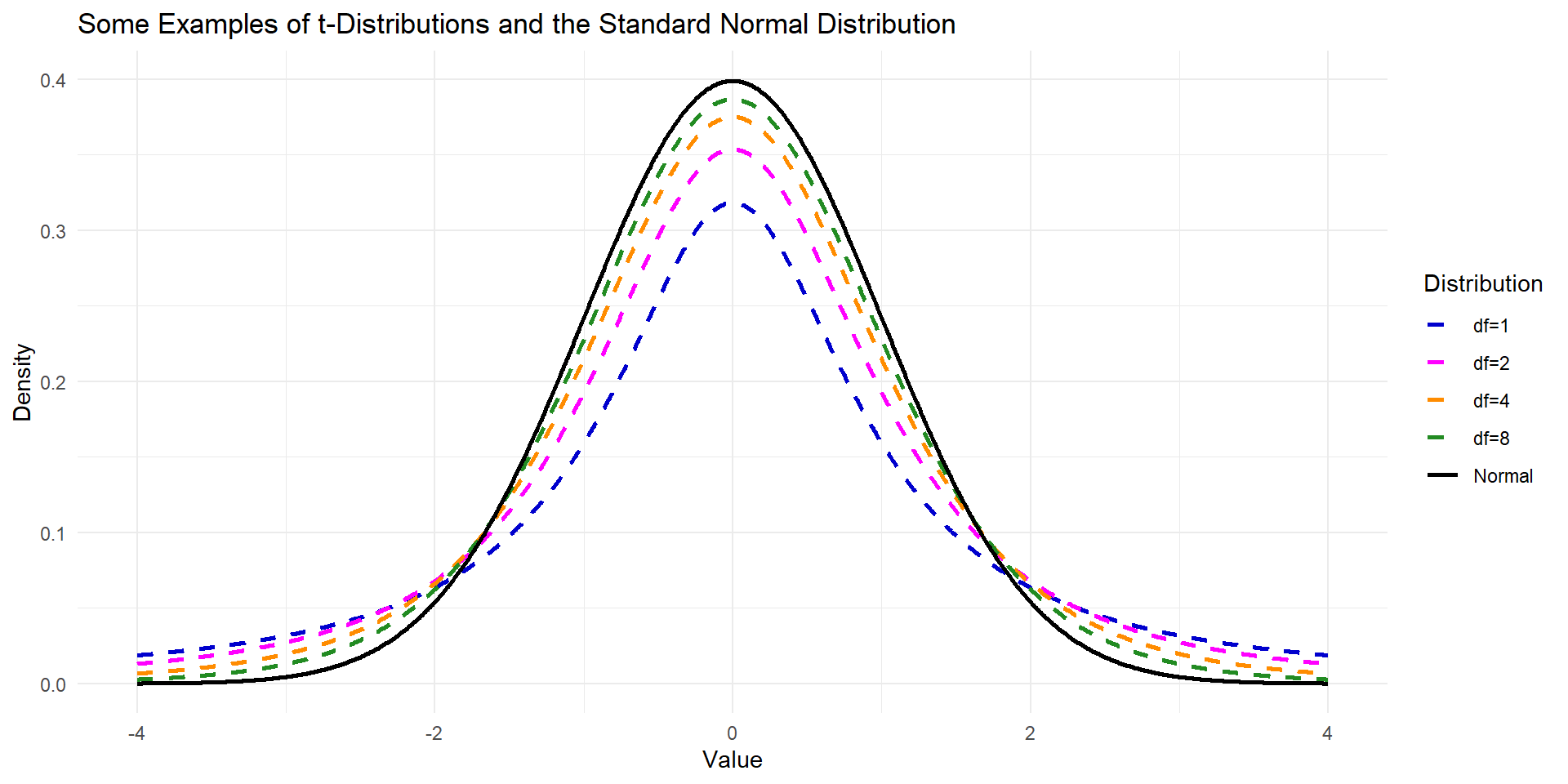
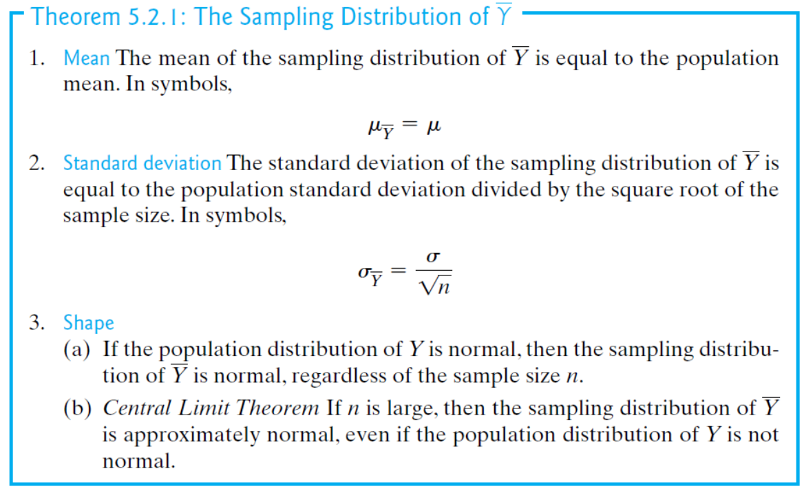
Central Limit Theorem fo Sample Means

Confidence Interval for µ

Introduction

In previous chapters, we were focusing on inferences about a population proportion (categorical variable).
Now, we will focus on data consisting of a single quantitative variable.
We will make inferences about a population mean (this is our new parameter now) by creating confidence intervals.

Confidence Interval Formula - Revisited

The general form of a confidence interval is

\[ \\ statistic \pm multiplier \times (SD \ of \ statistic) \]

Here, our statistic will be the sample mean and multiplier will come from t-distribution.

\[ \\ \bar{x} \pm t^* \times (s/ \sqrt{n}) \]

Student’s t distribution

What is t distribution?

\(t\)-distribution is another bell shape and symmetric distribution that can be useful if we do not know anything about population parameters.
The \(t\)-distribution is always centered at zero and has a single parameter: degrees of freedom.
- The shape of the distribution depends on the degrees of freedom.
Broadly speaking, we use \(t\)-distribution with \(df = n − 1\)
- to model the sample mean when the sample size is \(n\).
- As the \(df\) is increasing, the \(t\)-distribution will look more like the standard normal distribution
  - when the \(df\) is about 30 or more, the \(t\) -distribution is nearly indistinguishable from the normal distribution.

What is t distribution?

Comparison of t and the Standard Normal Distribution

Both are symmetric and bell-shaped but \(t\)-distribution has a larger standard deviation.
The \(t\)-distribution has a single parameter: degrees of freedom.
Standard Normal Distribution has two parameters: \(\mu\) and \(\sigma\).

Let’s Go Back to Confidence Interval

Monarch Butterflies - Example

Let’s have a look wing areas of 14 male Monarch butterflies at Oceano Dunes State Park in California

\(\bar{x} = 32.81\) \(cm^2\) and \(s= 2.48\) \(cm^2\)

Suppose we consider these 14 observations as a random sample from a population.

\(\mu\) = the (population) mean wing area of male Monarch butterflies in the Oceano Dunes region
\(\sigma\) = the (population) SD of wing area of male Monarch butterflies in the Oceano Dunes region

From the sample data we have, we can say that

32.81 is an estimate of \(\mu\).
2.48 is an estimate of \(\sigma\).

Monarch Butterfly - Example

Let’s have a look wing areas of 14 male Monarch butterflies at Oceano Dunes State Park in California

\(\bar{x} = 32.8143 \ cm^2\) and \(s= 2.4757 \ cm^2\)

For the multiplier, it is given as

\[ \\ multiplier = 2.160 \]

95% confidence interval (CI) for \(\mu\) can be calculated as following:

\(\bar{x} = 32.8143 \ cm^2\) and \(s= 2.4757 \ cm^2\)

\[ \\95 \% \ CI = (\bar{x} \pm multiplier \ \times \ SE_{\bar{x}}) \\95 \% \ CI = (32.8143 \pm 2.160 \ \times \ 2.4757 / \sqrt{14}) \]

\[ \\= 32.81 \pm 1.43 \\ 31.43 \ cm^2 < \mu < 34.2 \ cm^2 \\ OR \\ 95 \% \ CI = (31.43,34.2) \]

Monarch Butterfly - Example

90% confidence interval (CI) for \(\mu\) can be calculated as following (multiplier:1.771):

\(\bar{x} = 32.8143 \ cm^2\) and \(s= 2.4757 \ cm^2\)

\[ \\90 \% \ CI = (\bar{y} \pm multiplier \ \times SE_{\bar{x}}) \\90 \% \ CI = (32.8143 \pm 1.771 \ \times \ 2.4757 / \sqrt{14}) \]

\[ \\= 32.81 \pm 1.17 \\ 31.64 \ cm^2 < \mu < 33.98 \ cm^2 \]

What were the differences between 90% CI and 95% CI?

Confidence Interval - Verbal Explanation

And…

If we calculate confidence intervals for each of these 100 samples, we will find that around 95% of these intervals capture the true population mean.
We are 95% confident that the true population mean is in this confidence interval.

Planning a Study to Estimate μ

Before collecting data for a research study, it is wise to consider in advance whether the estimates generated from the data will be sufficiently precise.
- It can be painful indeed to discover after a long and expensive study that the standard errors are so large that the primary questions addressed by the study cannot be answered.
The precision with which a population mean can be estimated is determined by two factors:

the population variability of the observed variable Y, and
the sample size.

Planning a Study to Estimate μ

In some situations the variability of Y cannot, and perhaps should not, be reduced.
- For example, a wildlife ecologist may wish to conduct a field study of a natural population of fish; the heterogeneity of the population is not controllable and in fact is a proper subject of investigation.
On the other hand, it is often appropriate, especially in comparative studies, to reduce the variability of Y by holding extraneous conditions as constant as possible.
- For example, physiological measurements may be taken at a fixed time of day; tissue may be held at a controlled temperature; all animals used in an experiment may be the same age

What sample size will be needed?

Recall that

\[ SE_{\bar{x}} = \frac{s}{\sqrt{n}} \]

We can use this formula to determine our sample size as follows:

\[ Desired \ SE = \frac{Guessed \ SD}{\sqrt{n}} \]

Monarch Butterfly - Example

Suppose the researcher is now planning a new study of butterflies Monarch butterflies at Oceano Dunes State Park in California and has decided that it would be desirable that the SE be no more than \(0.4 \ cm^2\)

\(\bar{y} = 32.8143 \ cm^2\) and \(s= 2.4757 \ cm^2\)

\[ SE_{\bar{y}} = s / \sqrt{n} \]

\[ Desired \ SE = Guessed \ SD / \sqrt{n} \]

\[ \\Desired \ SE = 2.48 / \sqrt{n} \ \le 0.4 \\ n\ge 38.4 \] \[ \\ at \ least \ 39 \ butterflies \]

You may wonder how a researcher would arrive at a value such as \(0.4 \ cm^2\) for the desired SE. Such a value is determined by considering how much error one is willing to tolerate in the estimate of μ.